Monday, March 01. 2010
Particulate Swarms
![[Radar image of Sydney during the dust storm of September 2009.]](http://blog.fabric.ch/fabric/images/1350_1267480801_0.jpg)
Editors Note: File under Glacier / Island / Storm, a studio run by BLDGBLOG at Columbia University GSAPP. Storm edition.
———–
“It is time / It is time for / It is time for stormy weather” – The Pixies
Storms deal in simple materials: air, water (in various states), and other particulates, such as dirt or dust. Though, not unlike species swarming in nature (or microcosmic viruses for that matter), they assemble, grow, pulse, and respond to environmental conditions. All the while, luring other similar material into their agitated state. Storms move somewhat indifferently to us and often in spite of us. They are often predictable and just forecastable enough to tease those of us that want to know when, where, and how much. All of this is done through pattern play, and behavioral modeling at two-scales: the massive regional and continental airpsaces, and the molecular or particle-based scale. Storms work in cycles, some small seasonal cycles, some century long, and even some on significant larger timespans (quasi-periodic). We are looking here at three storms; all recurring, swirling, pulsing, and shifting–of various particulate matter: dust, water, nitrogen (air). This is through the filter of states of matter: solid, liquid, and gaseous.
![[Map showing plume expansion rate, dircetion and growth of the Australian dust storm of 2009.]](http://blog.fabric.ch/fabric/images/1350_1267480802_1.png)
1. Solid Storm: Dust // Certainly as one of the most fantastically documented storms of our young century, the Australian Dust Storm of 2009, you have no doubt seen the surreal images of highly saturated red and orange airspace. For this event, air particulate readings were about 15,400 micrograms per cubic meter. A typical day registers at about 50 micrograms, and a bushfire registers around 500 micrograms per cubic meter. It was thick. What was interesting though when this 2-day event rapidly escalated was that its long-term effects were somehow overlooked in favor of the evocative photography of a Mars-like outback. Within two weeks after the flash storm, scientists realized that the event caused a massive shift of phosphates and nitrogen as 4000 tons of desert topsoil particulates were dumped in the Sydney Harbour. Beyond that, the estimates for materials dumped in the Tasman Sea were an astounding 3,000,000 tons. And, as if a massive simulation of ocean fertilization, it was believed that this spurned phytoplankton growth to triple. So, what was in limited supply–yet was needed to grow life–in the desert ocean is ironically abundant in desert land. Further estimates put the additional phytoplankton in the Sea at 2 million tons, and, more impressively, with that about 8 million tons of CO2 captured. Eight million tons; thats a full months of a coal-fired power plant CO2 emission. Estimates for the amount of fish spawned from the increased phytoplankton are not known, but one can only imagine. Storms spawn swarms. Ocean fertilization inadvertently simulated at a massive scale by nature itself. Should it still be called geo-engineering if, in fact, it already occurs naturally on a massive?
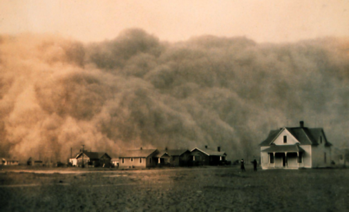
A note should also be included on the Dust Bowl of the 1930s, aka dirty thirties. The Dust Bowl phenomenon lasted during a drought in the Great Plains from 1930-36. After the dust had settled, it was shown that farming practices in the region were irresponsible with crop rotation, deep plowing, and erosion prevention. On numerous occasions during the dust clouds, the sky would turn black by day as far East as Washington DC. Dirt fell like snow in Chicago. The winter of 1934 red snow fell in the Northeast. And on April 24, 1935, the day became known as Black Sunday.
Some believe the Dust Bowl was predictable. Here is a PBS video on the Dust Bowl years.
Another interesting diversion on dust storms is the alkali storms found at Owens Lake and other salt flats. This is well documented by Barry Lehrman in The Infrastructural City. (Pruned has an excellent writeup on this here.)
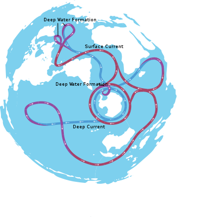
2. Liquid Storm: Water // One of the major circulatory systems responsible for the movement of large masses of water (and their associated species) and stabilizing the global climate is the Thermohaline Circulation (THC). The Thermohaline is an underwater storm–a massive global current. Known as the Great Ocean Conveyor, the Thermohaline Circulation is a series of underwater oceanic currents that are informed by the density of water, which is a function of the water’s temperature and salinity. Warm salty water is rapidly cooled as it reaches northern latitudes and as it forms into ice, sheds much of its salt. This increases the salinity in the remaining unfrozen cold water, making it denser and causing it to drop to the ocean floor (known as the ‘North Atlantic Deep Water’). This denser water moves towards the equator where it gains heat and migrates upwards. Global warming is promoting increased melting of the polar ice caps, leading to a more consistent density of water and slowing the thermohaline cycle. This has large potential effects on the climates of northern Europe and North America as well as destabilizing the sea ice formation in the arctic (and their associated ecosystems).
![[Trend Velocities in North Atlantic in meters per second per decade from May 1992 to June 2002. vectors trace the following graphic of the subpolar circulation in reverse direction, which denotes a slowing gyre. Credit: Sirpa Hakkinen, NASA GSFC.]](http://blog.fabric.ch/fabric/images/1350_1267480809_4.jpg)
The seasonal movement of the ice shelf constitutes one of the largest annual transformations in the Arctic and is the basis for the arctic ecosystem. As the summer months thaw the ice shelf, causing it to migrate northwards, fresh water is released into the sea. This freshwater promotes a blanket of fertile phytoplankton that forms the foundation of the arctic ecological food chain. Ecosystems that migrate with the annual retreat of ice traverse the Arctic seasonally. In the last 30 years, however, the summer sea ice extent has reduced by approximately 15 – 20%, while its average thickness has decreased by 10 – 15%. Both of these rates continue to increase, decreasing the foundation of the food chain and consequently applying pressure on species higher in the food chain.
Recent data points to something not-so-innocently called the Great Atlantic Shutdown. As increasing amounts of freshwater enter the THC water is more bouyant and less likely to sink, slowing or even stalling circulation.
![[The jet stream. The northern hemisphere polar jet stream is most commonly found between latitudes 30°N and 60°N, while the northern subtropical jet stream located close to latitude 30°N.]](http://blog.fabric.ch/fabric/images/1350_1267480811_5.jpg)
3. Gaseous Storm: Jet Stream // Winds have names: Katabatic, Foehn, Mistral, Bora, Cers, Marin, Levant, Gregale, Khamaseen, Harmattan, Levantades, Sirocco, Leveche, and many others (all exhaustively documented here). But all pale in comparison to the steady circulations of the tropospheric jet stream. The jet stream is a shifting river of air about 9-14 km above sea level that guides storm systems and cool air around the globe. And when it moves away from a region, high pressure and clear skies predominate. The jet stream marks a thick shifting swirling line that separates airspace that warms with height and airspace that cools with height. In short, it is the jet stream(s) that creates weather – all kinds of weather, from the ordinary, uninteresting dull gray sky to the devastating life-changing weather phenomenon.
The path of the jet typically has a meandering shape, and these meanders themselves propagate east, at lower speeds than that of the actual wind within the flow. Each large meander, or wave, within the jet stream is known as a Rossby wave. Rossby waves are caused by changes in the Coriolis effect with latitude, and propagate westward with respect to the flow in which they are embedded, which slows down the eastward migration of upper level troughs and ridges across the globe when compared to their embedded shortwave troughs.
![[The jet stream core region averages 160 km/h (100 mph) in winter and 80 km/h (50 mph) in summer. Those segments within the jet stream where winds attain their highest speeds are known as jet streaks.]](http://blog.fabric.ch/fabric/images/1350_1267480812_6.gif)
When the jet stream fractions off an eddy, such a minor event at the scale of the stream generates an cyclone as it hits the ground. Thought to be weakening and moving poleward, the jet stream would produce less rain in the south and more storms in the north. Though in the meantime, there is considerable ongoing research on how to harness this steady streaming power.
![[A wind machine, floated into the jet stream, would transmit electricity on aluminum or copper cables--or through invisible microwave beams--down to power grids, where it would be distributed locally.]](http://blog.fabric.ch/fabric/images/1350_1267480814_7.jpg)
One study (above) shows a range of kites responding to the stream in a variety of ways and at different altitudes. The possibility of a series of kites–ladder, rotor, rotating, or turntable–hovering 1000 feet in the air generating anywhere from 50- 250 kilowatts is hard to refute. Afterall, they are just kites. Or maybe, to test this possibility, we just need to tap into all the already ongoing leisurely kite-flying practices–so that regular kites are no longer available, but instead streaming kites only. Streaming kites flying much higher, and of course bigger, and equipped with gear that helps store and harness energy. At the end of a pleasurable day flying a kite you have next weeks electricity in a black box to tote back home.
Post inspired by: Star Archive, Storm Archive, Storm Control Authority, Meteorological Alchemy, Carcinogenic Storms, Life on Mars, Average Natures.
-----
Via InfraNet Lab
Personal comment:
Intéressant peut-être dans le contexte de notre projet orienté "storms & lightnings".
fabric | rblg
This blog is the survey website of fabric | ch - studio for architecture, interaction and research.
We curate and reblog articles, researches, writings, exhibitions and projects that we notice and find interesting during our everyday practice and readings.
Most articles concern the intertwined fields of architecture, territory, art, interaction design, thinking and science. From time to time, we also publish documentation about our own work and research, immersed among these related resources and inspirations.
This website is used by fabric | ch as archive, references and resources. It is shared with all those interested in the same topics as we are, in the hope that they will also find valuable references and content in it.
Quicksearch
Categories
Calendar
|
|
May '24 | |||||
| Mon | Tue | Wed | Thu | Fri | Sat | Sun |
| 1 | 2 | 3 | 4 | 5 | ||
| 6 | 7 | 8 | 9 | 10 | 11 | 12 |
| 13 | 14 | 15 | 16 | 17 | 18 | 19 |
| 20 | 21 | 22 | 23 | 24 | 25 | 26 |
| 27 | 28 | 29 | 30 | 31 | ||
